
Module 4: Case Studies & Examples
Using the Probability Calculator
For these case studies we will use the Probability Calculator included in your toolkit.
This calculator is very simple to use. You input the values for P(A) and P(B), and all the formulas are auto calculated.
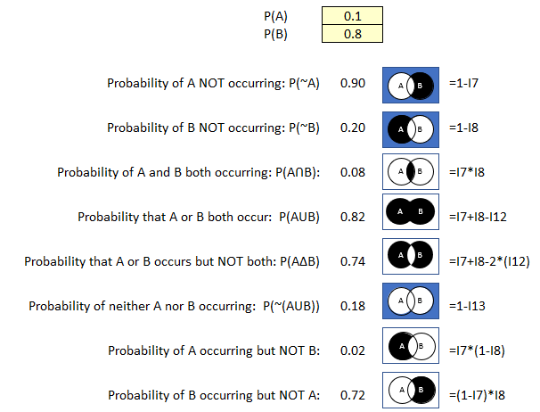
Figure 36 Probability Calculator Example 1
Malware Infection
You’ve been asked to provide an estimate of the risk of users downloading malicious software and it is resulting in damage or data loss. You spoke with operations and learned that while your perimeter defense and cybersecurity awareness training is quite good there are occasions where users have clicked links and downloaded malware. Operations agreed that it happens in less than 10% of the incidents they respond to, so you have agreed to use the estimate of 8%.
Next, you researched public statistics and found that 75% of malware is malicious, resulting in damage or data loss.
P(A): .08 (8% probability of a user downloading and executing malicious software)
P(B): .75 (75% of the malware causing system damage or data loss)
Now let’s see what else we can learn using our probability calculator and just these two inputs.
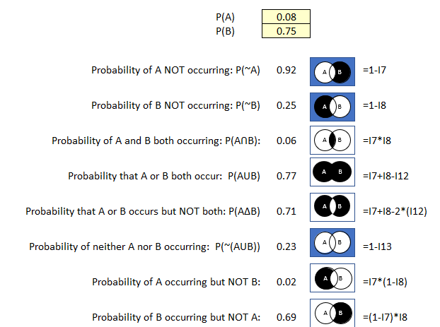
Figure 37 Probability Calculator Example 2
We are interested in the probability that users will (or will not) download malicious software, and that the malicious software once downloaded will (or will not) cause damage or loss.
- There is a 92% probability that users will not download malicious software.
- There is a 6% probability that users will download malicious malware that will result in damage and data loss.
- There is a 2% probability users will download malicious software but that it will not result in damage or data loss.
Ransomware Attack on Accounting
You’ve been asked to provide an estimate of risk for the following scenario:
A well-known and widely used accounting software is compromised by attackers so that when users of this software receive their next automatic update ransomware will be installed on their systems. Attackers successfully encrypt financial records, demanding a ransom for decryption.
You research public statistics and estimate that 35% of companies like yours in your industry use the same accounting software. You consider public statistics on ransomware trends in your industry and estimate a 25% probability of experiencing such an attack and decide to use that statistic for this scenario.
P(A): .35 (35% probability of the accounting software your company uses being compromised by hackers to deliver ransomware)
P(B): .25 (25% probability that your industry and your company could be targets of ransomware this year)
Let’s see what you can learn using just these two values and the probability calculator.
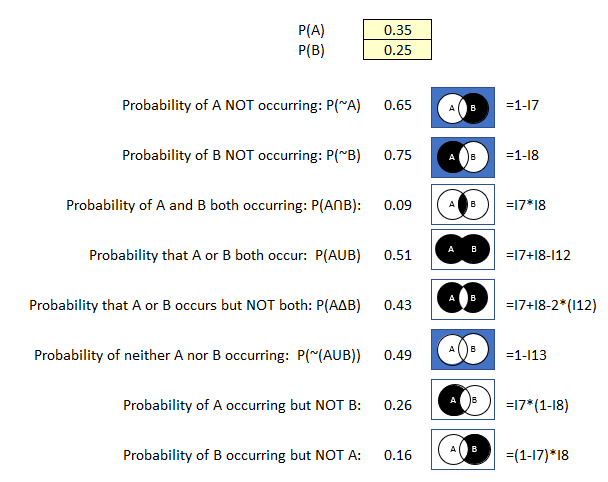
Figure 38 Probability Calculator Example 3
Based on the current industry data, you estimate the following:
- There is a 65 % probability that the accounting software isn’t compromised by attackers.
- There is a 9% probability that the account software is compromised and that your company is targeted resulting in data encryption for ransom.
- There is a 26% probability that the accounting software is compromised but that your company is not targeted for ransom.
Unauthorized Access to Cloud Storage
Your organization is considering investing in cloud-based data storage and there will be sensitive data involved. You are asked to provide an estimate for the following scenario: an employee accidentally shares a link to a sensitive cloud storage folder and an external party gains unauthorized access to confidential files.
You speak with operations and review the proposed controls and are impressed with the security and training that is planned. Share permissions will be restricted so you estimate a very low probability that users could accidentally share a link to sensitive data that could be shared to external parties. You estimate a 2% probability of this.
Next you estimate a slightly lower probability that external parties could access the confidential files. You estimate a 1% probability of this.
P(A): .02 (2% probability an employee could accidentally share a link to sensitive cloud storage folder)
P(B): .01 (1% probability an external party gains unauthorized access to confidential files).
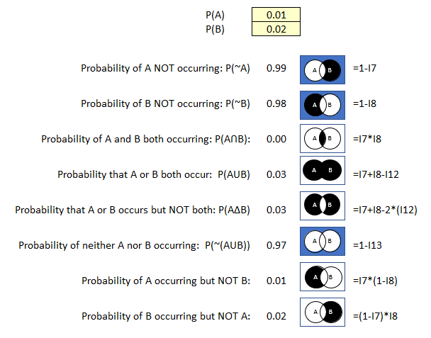
Figure 39 Probability Calculator Example 4
- There is a 99% probability employees could not share a link to sensitive cloud storage folder.
- The probability calculator only computes two decimal places, but with your calculator you multiple .01 * .02 as .000002 or .002% probability that an employee could share the link and that an external party could access the sensitive cloud data.
- There is a 1% probability an employee could share a link to the sensitive data.
While these probabilities are extremely small, sometimes it is important to be able to express these extremely unlikely probabilities because they could represent catastrophic impacts to the organization. We typically call these kinds of events “black swans”. They are extremely unlikely, but should they occur, they could have catastrophic impact on the organization.
Insider Threat of Data Exfiltration
You are asked to estimate the likelihood that an employee leaving the company would remove intellectual property.
You speak with human resources and learn that there has been a 30% turnover trend this year in the developer department, and you know that your company is working on a new product effort. You also research public statistics and learn that 15% of espionage (data exfiltration) in your industry occurs from disgruntled employees.
P(A): .3 (30% probability an employee with access to intellectual property planning to leave the company)
P(B): .15 (15% probability that a disgruntled employee would exfiltrate intellectual property)
Let’s see what you learn using the probability calculator.
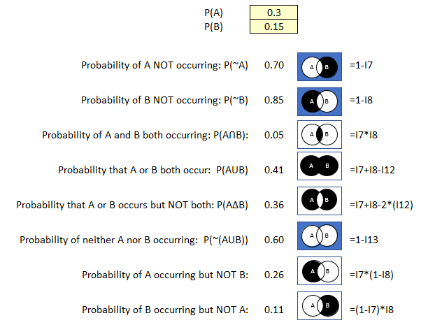
Figure 40 Probability Calculator Example 5
- There is a 70% probability of employees with access to intellectual property will not leave the company this year.
- There is a 5% probability that employees with access to intellectual property will leave the company this year and exfiltrate intellectual property when they go.
- There is a 26% probability of employees with access to intellectual property will leave the firm this year but will not exfiltrate intellectual property.
Probability Tree & Bayes’ Box
Phishing Attack
In this case study we are considering the probabilities of two events, receiving an email and experiencing a data breach. We will need to assign probabilities to all the resulting combinations as we put our data into the model.
We have the possibility of legitimate email or a phishing attempt. We’ll label these (Legit) and (Phish). We also have the possibility of a data breach or not. We’ll label these possible outcomes (Breach) and (NoBreach).
Let’s put some data into our probability tree model.
- (Legit) = .9 (90% probability incoming email will be legitimate)
- (Legit)+(NoBreach) =.95 (95% probability incoming email will be legitimate, and no breach will occur)
- (Legit)+(Breach)=.05 (5% probability incoming email will be legitimate, and a breach will occur)
- (Phish)=.1 (10% probability incoming email will be phishing attempt)
- (Phish)+(NoBreach) = .8 (80% probability incoming email will be phishing, and no breach will occur)
- (Phish)+(Breach) =.2 (20% incoming email will be phishing and a breach will occur)
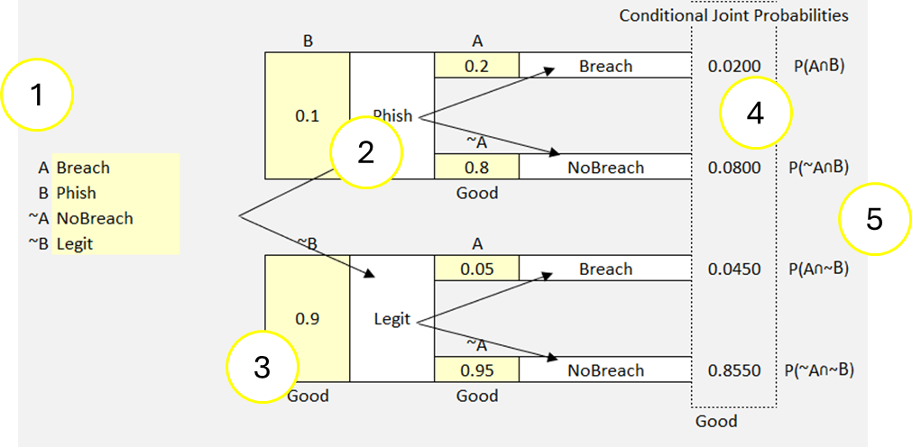
Figure 41 Probability Tree Example 1
Notice that when we input our labels (light yellow fields far left side) (1) the model auto-populates those labels across our tree (2). Next, we input our values (yellow fields in model (3). The model auto-calculates the joint probabilities (4). Notice (5) that the model also gives you the formulas for the joint probabilities. These formulas are also used in the Bayes’ box model.
The probability tree gives us two scenarios. One scenario begins with a legitimate email, the other begins with receipt of a phishing email. We can see the outcomes of each branch in both scenarios. We can see that the probability of a breach following a phishing attack is 2% P(A∩B), and that the probability of a breach without having received a phishing attack is 4.5% P(A∩~B).
Now let’s look to the right side of our model.
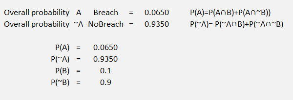
Figure 42 Probability Tree Example 1 Part 2
Remember that we labeled A, ~A, B and B. When we created the two scenarios (the two branches of the tree) we have different probabilities for A and ~A in each branch. Now we want to know the overall probability of a breach.
To get the overall probability of a breach P(A) we add the probability of a breach from both branched scenarios, and we get 2% + 4.5% = 6.5%. We can do the same to calculate the overall probability of not having a breach P(~A) and we get 93.5%.
Let’s use this same example with the Bayes’ box model.
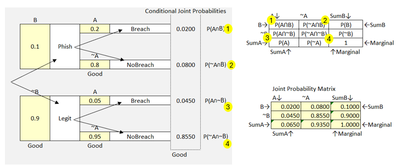
Figure 43 Probability Tree & Bayes’ Box Example
To the left we have our probability tree scenarios, and to the right we have Bayes’ box. From our probability tree we noted in the far-right column, the joint probabilities we calculated for each branch of the tree. Notice how these match the joint probabilities of the Bayes’ box model. Let’s use this to fill in the Bayes’ box model.
Recall that the power of Bayes’ is that it updates our probability with new data. We began our example with estimates of the probability of a data breach given receipt of a phishing email. Now when we carry our data forward into Bayes’ box we see the Bayesian formula updates our estimate.
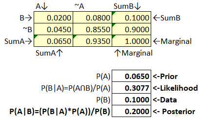
Figure 44 Bayes’ Box Example 1
Our prior belief (our overall probability of a data breach from the probability tree) was .0650.
Our new posterior (updated) probability is 0.20. That’s quite an increase for our estimate.
Let’s keep the same values again for data and likelihood and generate a new posterior. The purpose of this exercise is to explore the impact of changing the single value of A to explore if changing this value could lead to an improved estimate.
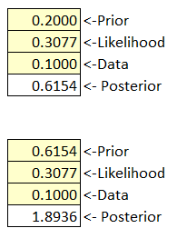
Figure 45 Bayes’ Box Iteration Example
As the posterior value increases and nears 1.0 it indicates the data supports the new prior P(A). If the posterior is greater than 1 you should either stop or make modifications to your data value.
You can collect new data (update our probability tree with adjusted values) or iterate using the existing data value to get a feel for a suitable range of P(A) values.
Firewall Rules
In this scenario, we’re going to explore probabilities using a firewall configuration. We will look at whether the firewall is configured correctly (or not), and whether there is likely to be an attack (or not).
Let’s use the following labels:
P(A) = Attack
P(~A) = NoAttack
P(B) = Incorrect configuration
P(~B) = Correct configuration
Now let’s add our probabilities:
- Correct Configuration (.8)
- No Attack (0.95)
- Attack (0.05)
- Incorrect Configuration (.20)
- No Attack (.70)
- Attack (.30)
Now let’s get this into the model.
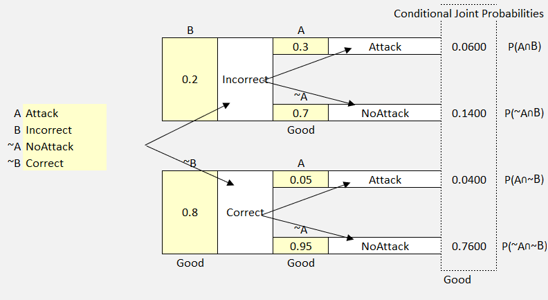
Figure 46 Probability Tree Example 2
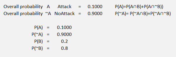
Figure 47 Probability Tree Example 2 Part 2
Given this data we see an overall 10% probability of an attack.
Now, let’s transform our data into a Bayes’ box model and see if we can improve our estimate.
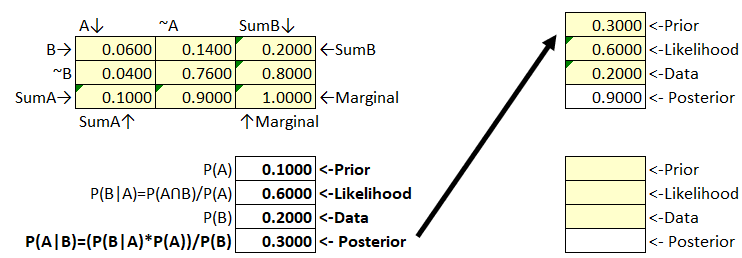
Figure 48 Bayes’ Box Example 2
In this example, our prior increased from .10 to .30. Using this new prior we get a .90 posterior. At this point there’s no need to iterate again. Given this information we should definitely consider updating our initial estimate of A.
But what if we were only concerned with a single scenario and set of probabilities?
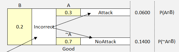
Figure 49 Detail View Probability Tree
We can still use the Bayes’ box and a single scenario of probabilities. Let’s take a look.
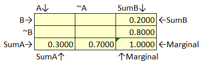
Figure 50 Bayes’ Box Example Step 1
In our single scenario we know that P(B)=.20 so we can deduce that P(~B)=1-P(B) or 1-.2 which is .80. Our single scenario gives us both P(A) and P(~A), so we can put those into the Bayes’ box. Now we just have to solve for the inner joint probabilities.
Let’s review the formulas for the inner joint probabilities.
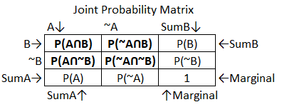
Figure 51 Bayes’ Box Example Step 2
Recall that joint probabilities are simple multiplication of the two probabilities involved.
Knowing this we can multiple P(B)*P(A) = .20*.3 = .060. We also know that P(A) is made up of the two component joint probabilities in the rows above it, so if we subtract P(AՈB) from P(A) we’ll solve for P(AՈ~B).
We also know P(B) is comprised of its subcomponent joint probabilities in the top row. We have solved P(AՈB), so we just subtract P(AՈB) from P(B) and get P(~AՈB).
Follow the same for P(~A) subcomponents.
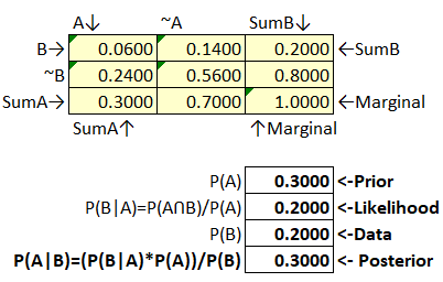
Figure 52 Bayes’ Box Example Step 3
The probabilities are independent so we will not get any additional value by attempting to iterate. What we do learn is that the probability of B given A is very low, and the probability of A given B is also very low. We should consider revising our initial estimate.
Software Vulnerabilities
For this example, let’s consider a software system with a vulnerability. A security patch can be applied (patch) or not (no patch).
Let’s set up our labels and initial estimates.
P(A) Exploit
P(~A) No Exploit
P(B) No Patch
P(~B) Patch
- Patch (.70)
- No Exploit (.90)
- Exploit (.10)
- No Patch (.30)
- No Exploit (.50)
- Exploit (.50)
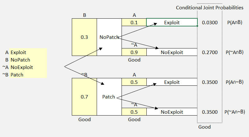
Figure 53 Probability Tree Example 3
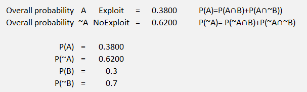
Figure 54 Probability Tree Example 3 Part 2
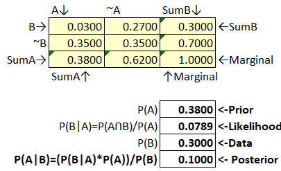
Figure 55 Bayes’ Box Example 3
This appears to be a very weak estimate for P(A) given P(B), and P(B|A).
