
Module 4: Terminology & Concepts
Making Decisions in the Face of Uncertainty
Uncertainty is a common aspect of life. We often face situations where we do not have all the information, we need to make a decision with complete confidence. Uncertainty can arise from various sources, including incomplete information, conflicting data, and unpredictable events. In such situations, we must learn to make decisions in uncertainty.
One approach to dealing with uncertainty is to eliminate the obvious. There will always be some extremes you can dismiss as highly unlikely or relevant. By eliminating the known unlikely options or values, you are left with more likely options. This begins to define a range of likely solutions or values. This approach is far more productive than beginning by saying you have “no idea” of the options. We are already closer to making more informed decisions based on a bit of logic.
The challenge with uncertainty is how to proceed toward a decision. You can apply a simple process that works every time to unravel that difficulty. We call this analysis. First, we must identify the problem or issue at hand. Once we have identified the problem, we must gather and evaluate relevant information. This involves researching and analyzing the available data to understand the situation better. We might consult experts, read reports, or conduct our own analysis to gather the necessary information. The goal is to reduce uncertainty by increasing our knowledge and understanding of the situation.
As part of information gathering and evaluation, we need to consider contributing factors and focus on those factors that impact possible outcomes. By again applying the process of elimination and removing factors that have no impact on the outcome, your efforts and analysis become more focused and effective.
We often consider uncertainty in the face of some “known.” For example, if we know that A is true, we might evaluate the probability or likelihood that B will occur or impact the outcome. This involves using statistical or other analytical methods to estimate the likelihood of different factors and possible outcomes based on the available data. For example, if we know that a particular medical treatment has been effective in 80% of cases, we might use this information to estimate the likelihood that the treatment will be effective for a particular patient.
Types of Events in Probability
In probability theory, there are several important conditions to consider when calculating the likelihood of an event occurring. The first condition is called conditional probability, which is the probability of an event occurring given that another event has already occurred. This powerful tool is used in various applications, from predicting medical test outcomes to analyzing complex systems’ performance.
Another important condition is independence, which refers to the relationship between two events. Two events are said to be independent if the occurrence of one event does not affect the probability of the other event occurring. For example, the probability of rolling a six on a fair die is independent of the outcome of any previous rolls.
In other words, independent events don’t reveal any information about the occurrence or non-occurrence of other events.
Independent events can happen separately or simultaneously and still be independent. Two events can be independent even if they have a cause-and-effect relationship. For example, consider the likelihood of running late in the morning and the likelihood of hitting a red light. These are two independent events that can happen at the same time, and red lights can make you late for work.
We can calculate whether or not two events are independent by comparing the product of their individual probabilities to the probability of their intersection (both events happening together). If this equation holds true, then events A and B are considered independent.
P(A∩B) = P(A) * P(B)
P(A|B) = P(A)
P(B|A) = P(B)
Notice that you have multiple values: P(A), P(B), P(A∩B), P(A|B), P(B|A). As you work with different scenarios for quantifying risk, you will be given some information. Depending on what information you have it may be very easy or quite difficult to determine whether two events are independent. Also, as you work through different scenarios it is important to be very clear about the events or conditions you define as A and B.
In contrast, two events are said to be dependent if the occurrence of one event affects the probability of the other event occurring. For example, the probability of getting a positive result on a medical test is dependent on the presence or absence of the disease being tested for.
In conditional probability, the words “and,” “or,” and “not” are used to describe the relationship between events. These words are used to construct logical statements that help us to calculate the probability of an event occurring, given that another event has already occurred.
The word “and” describes the intersection of two events. The word “or” describes the union of two events. The word “not” describes the complement of an event. The complement of event A is that which is not A, meaning it is the event where A does not occur.
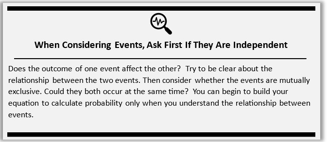
Figure 30 When Considering Events, First Ask If They Are Independent
Events are mutually exclusive if they cannot occur at the same time. This means that if one event occurs, the other event cannot occur. For example, “rolling a 1” and “rolling a 2” on a fair die are mutually exclusive because if the die rolls a 1, it cannot also roll a 2.
Mutually exclusive events are independent events that have no shared outcomes.
When events are mutually exclusive, the probability of either event occurring can be calculated by adding their individual probabilities. This is because the occurrence of one event precludes the occurrence of the other event.
The formula for calculating the probability of either event occurring is:
P(A or B) = P(A) + P(B)
Where P(A or B) is the probability of either event A or event B occurring, and P(A) and P(B) are the probabilities of events A and B occurring, respectively.
In contrast, events are said to be non-mutually exclusive if they can occur at the same time. This means that if one event occurs, the other event can still occur. For example, the events “rolling an even number” and “rolling a number greater than 2” on a fair die are non-mutually exclusive because if the die rolls a 2, it satisfies both events.
When events are non-mutually exclusive, the probability of either event occurring is calculated by adding their individual probabilities and subtracting the probability of both occurring. This is because the probability of both events occurring together is counted twice when we add the individual probabilities. The formula for calculating the probability of either event occurring is:
P(A or B) = P(A) + P(B) – P(A and B)
Where P(A or B) is the probability of either event A or event B occurring, P(A) and P(B) are the probabilities of events A and B occurring, respectively, and P(A and B) is the probability of both events A and B occurring together.
Events are mutually exclusive if they cannot occur at the same time, while events are non-mutually exclusive if they can occur at the same time. The probability of either event occurring is calculated differently depending on whether the events are mutually exclusive or non-mutually exclusive.
Some Basic Probability Equations
Probability of A NOT Occurring: P(~A)
In probability theory, the probability of an event A not occurring, denoted as P(~A), equals 1 minus the probability of event A occurring, denoted as P(A). That is:
P(~A) = 1 – P(A)
If events A and ~A are mutually exclusive, then either A occurs, or ~A occurs, but not both. In this case, the sum of their probabilities equals 1 since one of the events must occur. That is:
P(A) + P(~A) = 1
Therefore, we can use the equation P(~A) = 1 – P(A) to calculate the probability of event ~A occurring if we know the probability of event A occurring. This equation is often used in probability calculations to simplify the calculation of probabilities by focusing on one event rather than both events.
For example, if the probability of a network intrusion occurring is 0.2, then the probability of a network intrusion not occurring is:
P(~network intrusion) = 1 – P(network intrusion) = 1 – 0.2 = 0.8
This means there is an 80% chance that a network intrusion will not occur. If the events “network intrusion” and “~network intrusion” are mutually exclusive, then we can use this probability to calculate the probability of a different event occurring instead of calculating the probability of both events occurring together.
Probability of B NOT Occurring: P(~B)
In probability theory, the probability of an event B not occurring, denoted as P(~B), equals 1 minus the probability of event B occurring, denoted as P(B). That is:
P(~B) = 1 – P(B)
If events B and ~B are mutually exclusive, then either B occurs, or ~B occurs, but not both. In this case, the sum of their probabilities equals 1 since one of the events must occur. That is:
P(B) + P(~B) = 1
Therefore, we can use the equation P(~B) = 1 – P(B) to calculate the probability of event ~B occurring if we know the probability of event B occurring. This equation is often used in probability calculations to simplify the calculation of probabilities by focusing on one event rather than both events.
For example, if the probability of a system being compromised due to a software vulnerability is 0.3, then the probability of the system not being compromised due to the same vulnerability is:
P(~compromise due to vulnerability) = 1 – P(compromise due to vulnerability) = 1 – 0.3 = 0.7
This means there is a 70% chance that the system will not be compromised due to the vulnerability. If the events “compromise due to vulnerability” and “~compromise due to vulnerability” are mutually exclusive, then we can use this probability to calculate the probability of a different event occurring instead of calculating the probability of both events occurring together.
Probability of A and B Both Occurring: P(AՈB)
In probability theory, the probability of events A and B both occurring, denoted as P(A∩B) or P(A and B), can be calculated using the formula:
P(A∩B) = P(A) * P(B|A)
Where P(A) is the probability of event A occurring, and P(B|A) is the conditional probability of event B occurring given that event A has occurred.
If events A and B are mutually exclusive, then they cannot occur at the same time. In this case, the probability of both events occurring together is zero since both events cannot occur simultaneously. That is:
P(A∩B) = 0
Therefore, the probability of events A and B both occurring, denoted as P(AՈB), is simply the sum of their individual probabilities since there is no overlap between the events. That is:
P(AՈB) = P(A) + P(B)
This equation holds only for mutually exclusive events. If events A and B are not mutually exclusive, then the probability of both events occurring together must take into account the overlap between the events, and the formula for calculating P(AՈB) becomes:
P(AՈB) = P(A) + P(B) – P(A∩B)
Where P(A∩B) is the probability of events A and B both occurring, taking into account the overlap between the events.
In summary, if events A and B are mutually exclusive, then the probability of both events occurring together is zero, and the probability of either event occurring is simply the sum of their individual probabilities. If events A and B are not mutually exclusive, then the probability of either event occurring must take into account the overlap between the events.
Probability That A or B Both Occur: P(AUB)
In probability theory, the probability of events A or B both occurring, denoted as P(A∪B) or P(A or B), can be calculated using the formula:
P(A∪B) = P(A) + P(B) – P(A∩B)
Where P(A) is the probability of event A occurring, P(B) is the probability of event B occurring, and P(A∩B) is the probability of events A and B both occurring.
If events A and B are mutually exclusive, then they cannot occur at the same time. In this case, the probability of both events occurring together is zero since both events cannot occur simultaneously. That is:
P(A∩B) = 0
Therefore, the formula for calculating P(A∪B) becomes:
P(A∪B) = P(A) + P(B)
This equation holds only for mutually exclusive events. If events A and B are not mutually exclusive, then the probability of both events occurring together must take into account the overlap between the events, and the formula for calculating P(A∪B) becomes:
P(A∪B) = P(A) + P(B) – P(A∩B)
Where P(A∩B) is the probability of events A and B both occurring, taking into account the overlap between the events.
In summary, if events A and B are mutually exclusive, then the probability of both events occurring together is zero, and the probability of either event occurring is simply the sum of their individual probabilities. If events A and B are not mutually exclusive, then the probability of either event occurring must take into account the overlap between the events. The formula for calculating P(A∪B) depends on whether the events are mutually exclusive or not.
Probability That A or B Occurs but NOT Both: P(A∆B)
In probability theory, the probability of events A or B occurring but not both, denoted as P(A∆B) or P(A exclusive or B), can be calculated using the formula:
P(A∆B) = P(A) + P(B) – 2P(A∩B)
Where P(A) is the probability of event A occurring, P(B) is the probability of event B occurring, and P(A∩B) is the probability of events A and B both occurring.
If events A and B are mutually exclusive, then they cannot occur at the same time. In this case, the probability of both events occurring together is zero since both events cannot occur simultaneously. That is:
P(A∩B) = 0
Therefore, the formula for calculating P(A∆B) becomes:
P(A∆B) = P(A) + P(B)
This equation holds only for mutually exclusive events. If events A and B are not mutually exclusive, then the probability of both events occurring together must take into account the overlap between the events, and the formula for calculating P(A∆B) becomes:
P(A∆B) = P(A) + P(B) – 2P(A∩B)
Where P(A∩B) is the probability of events A and B both occurring, taking into account the overlap between the events.
The formula for calculating P(A∆B) is used to find the probability that event A or event B occurs, but not both. This is sometimes referred to as the “exclusive or” probability. If events A and B are mutually exclusive, then the probability of both events occurring together is zero, and the exclusive probability is simply the sum of their individual probabilities. If events A and B are not mutually exclusive, then the exclusive or probability must take into account the overlap between the events.
Probability of Neither A nor B Occurring: P(~(AUB))
In probability theory, the probability of neither event A nor event B occurring, denoted as P(~(A∪B)) or P(neither A nor B), can be calculated using the formula:
P(~(A∪B)) = 1 – P(A∪B)
Where P(A∪B) is the probability of events A or B occurring.
If events A and B are mutually exclusive, then they cannot occur at the same time. In this case, the probability of either event occurring is simply the sum of their individual probabilities, and the probability of neither event occurring is:
P(~(A∪B)) = 1 – P(A) – P(B)
This equation holds only for mutually exclusive events. If events A and B are not mutually exclusive, then the probability of either event occurring must take into account the overlap between the events, and the formula for calculating P(~(A∪B)) becomes:
P(~(A∪B)) = 1 – P(A) – P(B) + P(A∩B)
Where P(A∩B) is the probability of events A and B both occurring, taking into account the overlap between the events.
In summary, if events A and B are mutually exclusive, then the probability of neither event occurring is simply one minus the probability of either event occurring. If events A and B are not mutually exclusive, then the probability of neither event occurring must take into account the overlap between the events. The formula for calculating P(~(A∪B)) depends on whether the events are mutually exclusive or not.
Probability of A Occurring but NOT B
In probability theory, the probability of event A occurring but not event B, denoted as P(A and not B) or P(A∩~B), can be calculated using the formula:
P(A and not B) = P(A) – P(A∩B)
Where P(A) is the probability of event A occurring, and P(A∩B) is the probability of events A and B both occurring.
If events A and B are mutually exclusive, then they cannot occur at the same time. In this case, the probability of both events occurring together is zero since both events cannot occur simultaneously. That is:
P(A∩B) = 0
Therefore, the formula for calculating P(A and not B) becomes:
P(A and not B) = P(A)
This equation holds only for mutually exclusive events. If events A and B are not mutually exclusive, then the probability of both events occurring together must take into account the overlap between the events, and the formula for calculating P(A and not B) becomes:
P(A and not B) = P(A) – P(A∩B)
where P(A∩B) is the probability of events A and B both occurring, taking into account the overlap between the events.
If events A and B are mutually exclusive, then the probability of event A occurring but not event B is simply the probability of event A occurring. If events A and B are not mutually exclusive, then the probability of event A occurring but not event B must take into account the overlap between the events. The formula for calculating P(A and not B) depends on whether the events are mutually exclusive or not.
Probability of B Occurring but NOT A
In probability theory, the probability of event B occurring but not event A, denoted as P(B and not A) or P(B∩~A), can be calculated using the formula:
P(B and not A) = P(B) – P(A∩B)
Where P(B) is the probability of event B occurring, and P(A∩B) is the probability of events A and B both occurring.
If events A and B are mutually exclusive, then they cannot occur at the same time. In this case, the probability of both events occurring together is zero since both events cannot occur simultaneously. That is:
P(A∩B) = 0
Therefore, the formula for calculating P(B and not A) becomes:
P(B and not A) = P(B)
This equation holds only for mutually exclusive events. If events A and B are not mutually exclusive, then the probability of both events occurring together must take into account the overlap between the events, and the formula for calculating P(B and not A) becomes:
P(B and not A) = P(B) – P(A∩B)
Where P(A∩B) is the probability of events A and B both occurring, taking into account the overlap between the events.
If events A and B are mutually exclusive, then the probability of event B occurring but not event A is simply the probability of event B occurring. If events A and B are not mutually exclusive, then the probability of event B occurring but not event A must take into account the overlap between the events. The formula for calculating P(B and not A) depends on whether the events are mutually exclusive or not.
Conditional Probability
Conditional probability refers to the possibly of an event occurring because another event has already previously occurred. We estimate these probabilities either as assumptions to be proven, or based on evidence available. The formulas for conditional probability involve the multiplication of a probability of the previous event (B) by the chances of the next event (A) occurring.
Conditional events are different from independent and mutually exclusive events.
Conditional probability tells us about the likelihood of an event occurring based on the conditions created from the previous event.
P(A)=P(A|B) is a basic conditional probability formula. We read it as the probability of A is equal to the probability of A given event B.
This symbol, the vertical bar “|” is used to denote conditional probability.
Bayesian inference is a statistical method for updating the probability of an event based on new information. It is a powerful tool for risk quantification because it allows for incorporating prior knowledge and experience into the analysis.
All Bayesian formulas represent conditional probabilities. These probabilities can involve independent or dependent events.
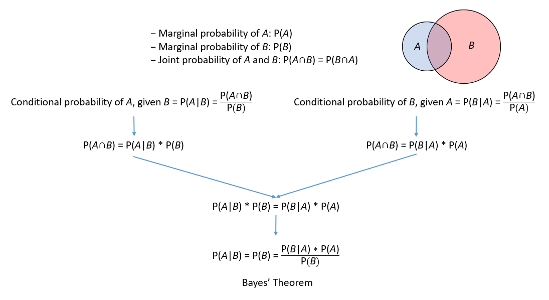
Bayesian inference involves using Bayes’ theorem, which states that the probability of an event given some evidence is proportional to the probability of the evidence given the event multiplied by the prior probability of the event. Mathematically, this can be expressed as:
P(A|B) = P(B|A) * P(A) / P(B)
where P(A|B) is the probability of event A given evidence (or observation) B, P(B|A) is the probability of evidence (or observation) B given event A, P(A) is the prior probability of event A, and P(B) is the probability of evidence B.
Bayesian evaluates two probabilities: A and B. It also considers their inverse or ~A and ~B (the ~ symbol means not).
You are given two models for working with Bayesian formulas. Both are designed to make it easy to understand and ensure your formulas are correct because they both use visual layouts and include auto-calculated formulas.
The strength of Bayesian inference is that you can infer, or logically deduce what we don’t know from data that we have. Using multiple Bayesian formulas, each updated to the next, allows us to systematically refine an initial estimate, becoming more precise in our forecasting.
Bayes’ Theorem
Bayes’ Theorem is named after the 18th-century British mathematician Thomas Bayes and is the mathematical expression of how we learn. Basically, it means that we start with a belief, which we update with new data. This powerful concept is at the heart of all AI learning algorithms.
Basically, Bayes’ Theorem describes the conditional probability of an event based on prior knowledge of conditions that might be relevant to the event.
We think of P(A) as our prior belief, our current understanding or prior knowledge. When new evidence is available, we consider it given our current belief P(B|A). This evidence could be anything relevant to P(A). Then we update our original belief with the evidence which we express as P(A|B) also called our posterior belief.
A key insight of Bayes’ Theorem is the swap in the order of cause and effect. Instead of directly calculating the probability of evidence given the event P(B|A), it calculates the probability of the event given the evidence P(A|B). This swaps allows you to incorporate new information into our beliefs. If the evidence strongly supports the initial belief, the updated probability will be high. If the evidence contradicts the initial belief, the updated probability will be lower.
Bayesian Inference
Inference refers to drawing conclusions or making judgments based on evidence, reasoning, and prior knowledge. Inference involves using available information to make educated guesses or predictions about something that is not directly observed or known. It is a key component of critical thinking and problem-solving in many fields, including science, mathematics, and everyday life. Inference can be based on deductive reasoning (starting with general principles and applying them to specific situations) and inductive reasoning (starting with specific observations and drawing general conclusions from them).
Bayesian inference is a statistical method used to update the probability of a hypothesis as new evidence or data becomes available. It involves calculating the posterior probability of a hypothesis by combining prior knowledge or beliefs with the likelihood of the observed data.
Bayes’ formula is the mathematical expression used to calculate the posterior probability of a hypothesis. It is represented as:
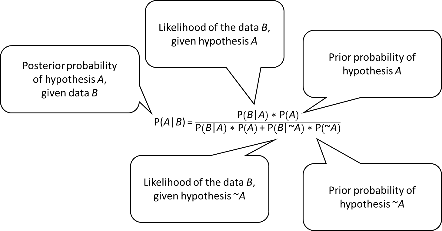
Where:
P(A|B) is the posterior probability of hypothesis A given the observed data B
P(B|A) is the likelihood of observing data B given hypothesis A
P(A) is the prior probability of hypothesis A
P(B) is the probability of observing data B
Bayes’ Formula allows us to update our beliefs about a hypothesis based on new evidence or data.
Independent and Dependent Events in Bayes
We can use independent or dependent events in Bayes’ formula. How can we tell the difference? If you don’t know how the events were generated or if you’re unsure whether they are actually independent or dependent, you can use the following equations to verify.
If A and B are the outcome of dependent events, then.
P(AՈB)=P(A)*P(B|A)
and thus P(B|A)= P(AՈB)/(PA)
If A and B are the outcomes of independent events, then.
P(B|A)=P(B)
and P(AՈB)=P(A)*(B)
Bayes’ formula will produce new posterior when you are using dependent events. One of the ways to know you are dealing with independent events is when the Bayes’ box doesn’t produce a new posterior value. So how can you get the benefit of Bayes’ new posterior when you are dealing with independent events?
Prior, Posterior and Likelihood
Bayesian provides us a means to improve our estimates by using the prior, posterior and likelihood. Like adjusting dials, these three values tell us when our estimates are realistic.
They are mathematically linked to reflect accuracy.
Likelihood P(B|A)=P(AՈB)/P(A) and posterior P(A|B)=P(AՈB)/P(B).
Note: these are the equations for dependent events.
Consider the basic equation P(AՈB) which is the joint probability, a basic multiplication of both the data P(B) and our estimate of the outcome P(A) based on observing that data. Likelihood and posterior simply divide the joint probability by the opposite value.
Likelihood tells us how realistic it is to actually observe P(B) given our estimate of P(A), and the posterior tells us how realistic it is to expect P(A) to happen given our estimate of P(B).
If the posterior exceeds 1 it means the values are not believable. It violates the fundamental norming axiom of probability theory, which simply states that the sum of probabilities adds to 1.
If the posterior is unexpectedly large, consider adjusting the prior by obtaining new data.
Each iteration should improve the accuracy of the posterior, based on accumulated evidence.
When we are estimating, modeling possible future events, we aren’t actually “observing events” we are observing our estimates in order to improve their accuracy.
Equations and Forms
It turns out that there can be several ways to write a formula expressing the relationship between two events. Depending on the situation, and what data you have available, you will select one form over another. This is both beneficial while possibly being a bit confusing. To ease the situation, the tools provided have several different forms presented so that you can more easily select the form best suited to the data available.
The Bayesian Box
An easy visual method for calculating probabilities is called the “Bayesian Box”. It is a simple probability matrix, that we use to solve Bayesian formulas. Values run down columns and across rows. The value A is found in the left-most column. It has two components on the first two rows, and its total value is the bottom row in the left-most cell P(A).
Here is a quick cheat sheet to help identify all the boxes and their values. P(~A∩B) is the same as P(B∩~A), for example, so solve for whichever expression is relevant. Notice that all we did was transpose the location of B and ~A in the equations, but both are the intersection of ~A and B. Find the box that represents P(~A∩B).
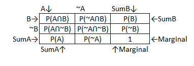
Figure 33 Bayes’ Box Internal Formulas
Notice that A is the sum of the first left-hand column P(A∩B) and P(A∩~B).
Notice that P(~A) is the sum of the middle column P(~A∩B) and P(~A ∩~B).
Notice that P(A) and P(~A) = 1
Notice that P(B) is the sum of the top row P(A∩B) and P(~A∩B).
Notice that P(~B) is the sum of the second row P(A∩~B) and P(~A∩~B).
Notice that P(B) and P(~B) = 1
You should notice that P(~B) = 1-P(B) and that P(B)=1-P(~B). The same is true for P(A) and P(~A).
The following are joint probabilities of the column and row A, ~A, B or ~B values:
P(A∩B), P(~A∩B), P(A∩~B), and P(~A∩~B). Joint probabilities represent multiplication of the two values. So, P(A∩B) is A*B, P(~A∩B) is ~A*B, P(A∩~B) is A*~B, and P(~A∩~B) is ~A*~B.
To easily solve the box, you need to know 3 of the following values A, ~A, B or ~B and one of the joint probabilities containing two of the 3 known values.
Marginal probability refers to the probability of a single event occurring without taking into account any other events. It is calculated by summing or integrating the joint probabilities of the event of interest with respect to all other events. In other words, the marginal probability is the probability of one variable occurring, regardless of the values of other variables. It is often used in probability theory and statistics to calculate the probability of a particular outcome in a multi-dimensional distribution.
Figure 34 How We Use Bayes’ Box Model
Conjoint probability, also known as joint probability, refers to the probability of two or more events occurring together. It is the probability of the intersection of two or more events and is calculated by multiplying the probabilities of each individual event. In other words, it is the likelihood of two or more things happening at the same time. Conjoint probability is often used in probability theory and statistics to calculate the probability of a particular outcome in a multi-dimensional distribution.
Three Bayesian Values
Bayesian inference is primarily concerned with three values, the prior believe P(A), the posterior believe P(A|B) the probability of A occurreing given the ocurrence of B.
Between the prior and posterior we calculate likelihood P(B|A). Notice that this is the opposite of P(A|B) or the probability of A given that B occurred. Instead, likelihood is the probability of observing the preciptating event P(B) given that our believe in P(A) is true.
One way to generate these three Bayesian values is to use the probability tree model.
Probability Trees
Probability trees, or decision trees, are a graphical representation of a decision-making process involving uncertainty. They are used to calculate joint probabilities, which are the probabilities of multiple events occurring simultaneously.
Use the probability tree when you are considering two events. In the graphical layout of the tree, the branches represent different possible outcomes of a decision or event. Each branch is labeled with the probability of that outcome occurring. The tree is constructed so that the probabilities of all possible outcomes sum to 1. The branches can be organized in a hierarchical structure, with each level of the tree representing a different stage of the decision-making process.
For example, consider the simple decision-making process of bringing an umbrella based on the weather forecast.

Figure 35 Probability Tree Example
Using this probability tree, we can calculate the joint probabilities of different outcomes. For example, the probability of it being sunny and bringing an umbrella (Sunny and Bring Umbrella) is the product of the probabilities of each individual outcome:
P(Sunny and Bring Umbrella) = P(Sunny) * P(Bring Umbrella | Sunny) = 0.7 * 0.3 = 0.21
Similarly, the probability of it not being sunny and not bringing an umbrella (Not Sunny and Do not Bring Umbrella) is the product of the probabilities of each individual outcome:
P(Not Sunny and Don’t Bring Umbrella) = P(Not Sunny) * P(Don’t Bring Umbrella | Not Sunny) = 0.3 * 0.7 = 0.21
Note: Recall that when we use “and” we are multiplying the values, as with a joint probability.
Probability trees can also be used to calculate conditional probabilities, which are the probabilities of an event occurring given that another event has already occurred. For example, we can use the probability tree above to calculate the probability of bringing an umbrella given that it is sunny:
P(Bring Umbrella | Sunny) = P(Sunny and Bring Umbrella) / P(Sunny) = 0.21 / 0.7 = 0.3
This conditional probability represents the probability of bringing an umbrella, given that we know it is sunny.
Probability trees can be extended to more complex decision-making processes, with multiple stages and multiple possible outcomes at each stage. They can also be used to represent probabilistic models, such as Bayesian networks, which are graphical models that represent the dependencies between variables and their probabilities.
