
Module 5: Case Studies & Examples
Example FAIR™ Analysis for Consideration of New Firewall Purchase
In this simple scenario, the company is considering the purchase of a new firewall. Note that secondary loss is not considered.
Threat Event Frequency
The company experiences an average of 10 attempted cyber-attacks per week.
Of those 10 attempts, the existing router blocks 7, meaning 30% of attacks get past the router.
Loss Magnitude
The cost of the existing router is $5,000.
The estimated cost of a new firewall is $15,000.
Based on industry research, implementing a new firewall is expected to reduce malicious traffic by 80%, bringing the 3 events down to (3-(3*.8) or 3-2.4=0.6 events.
The company currently spends an average of $10,000 per incident response.
The current cost is 3 events x $10,000/ea. = $30,000.
Expected new cost is 0.6 events x $10,000 = $6,000.
Savings of $24,000.
Modeling the risk
We will use the single digit values as most-likely estimates in a set of range values for the FAIR model.
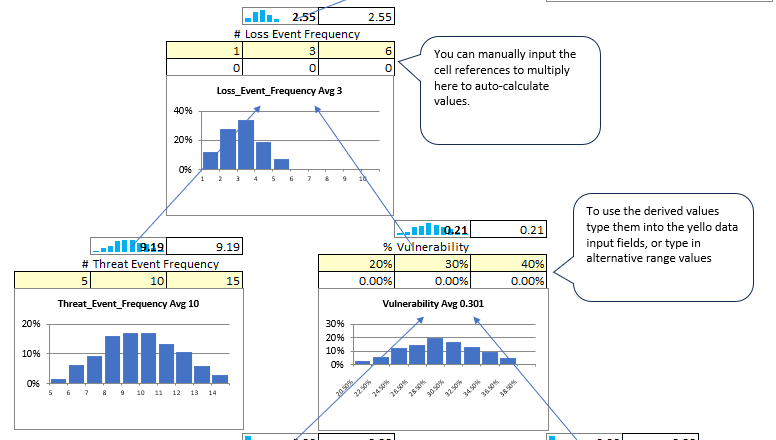
In this scenario, we only need to input the Threat Event Frequency and Vulnerability % values to calculate the Loss Event Frequency. Notice that the average threat event frequency is 10, the average vulnerability is .301 or 30% and the average loss event frequency is 3. These are the most-likely values from our single digit estimates.
For the financial portion, we need only input the Loss Magnitude.
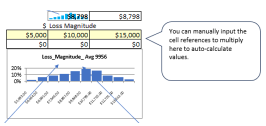
Figure 72 FAIR Example 1 Part 2
Our average loss magnitude is $9,956 which is in line with our single digit estimate of $10,000.
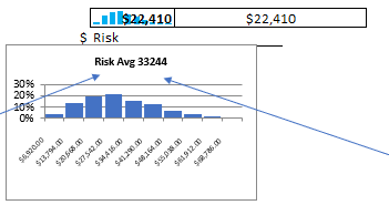
Figure 73 FAIR Example 1 part 3
The risk is then calculated, and the average risk is $33,244, again in line with our single digit estimate.
Remember that the $22,410 displayed at the top of this image is just 1 of the 1,000 values generated in the probability distribution. If you scroll through all 1,000 possibilities, you will see this number change to display all the values represented in the chart.
Example FAIR ™ Analysis Data Breach
In this scenario a consulting company has 2 offices, one on the east coast and one on the west coast. Each office has an exchange server, a share point server, perimeter defenses and 10 people per office. They use Office 365, and a variety of other applications. The company applies industry best practices and on average it takes 32 days to apply critical patches. What’s the risk that one of these will be leveraged against the company in the next 12 months and if the company breached estimate 5,000 records compromised at a cost of $135 per record.
Given this description you estimate internal control strength at 70%. They tend to accept default configurations on systems adding role-based access controls to sensitive data. They have a good internet provider which provides them with perimeter defense, and they have very good configurations on their firewalls and routers. Taking into account the internet provider’s protection you adjust the overall strength to 95% +/- 10%.
On average their host-based protections (anti-virus and firewall) report 5 files quarantined per month. You use this statistic to estimate threat event frequency at 60 per year (5*12=60) +/- 10%.
You estimate loss magnitude at 5,000 records * $135/record = $675,000 +/- 10%.
Let’s put this into the FAIR Model.
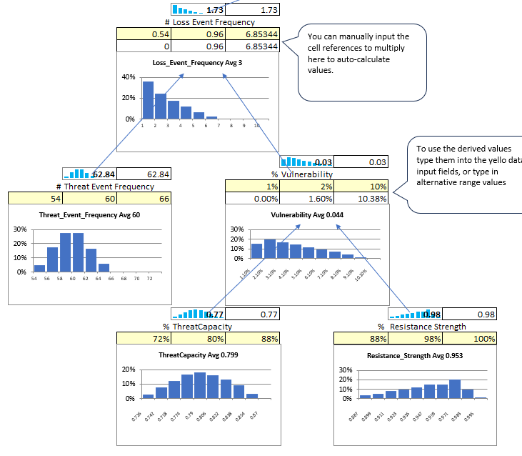
Figure 74 FAIR Example 2 Part 1
This is the loss event side of the model. What we are seeing in our scenario is that the resistance strength is primarily the internet provider perimeter defense and a strong end-point product. Should either of these fail or be breached the likelihood of compromise increases substantially. We refer to this as brittle security. We see this is the average estimate of loss event of 0.96, but the range allows the upper limit to be as high as 6.8. Notice that the vulnerability probability distribution is heavily skewed to the left, with a long tail to the right (far less likelihood of the higher value).
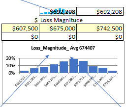
Figure 75 FAIR Example 2 Part 2
Loss magnitude is easy to calculate. You can use formulas in the minimum and maximum fields for the +/- 10% calculations.
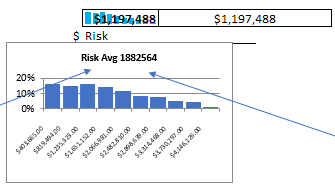
Figure 76 FAIR Example 2 Part 3
The average likely loss is $1,882,564. This reflects the +/- 10% of our estimate.
