Module 5: Terminology & Concepts
Monte Carlo Simulations – a Brief History
Monte Carlo Simulation is a numerical process used to estimate probabilities where there is uncertainty. The method works by complex algorithms that generate thousands of random values within the range you stipulate. These values are then also charted in a probability distribution chart. We use a 3-point value for the range so that there is a minimum, most likely, and maximum range. The most likely value can be used to skew or shape the distribution to the right or left as you so desire.
The method was invented during World War II by mathematicians Stanislaw Ulam and John von Neumann. They developed it while working on the Manhattan Project to simulate chain reactions in highly enriched uranium.
Ulam and von Neumann used random sampling and statistics to speed up calculations and make predictions. The technique was named “Monte Carlo” after the famous casino in Monaco.
There are several types of probability distributions, which we will discuss momentarily, but each has a specific intended purpose. For each, the math has been created to measure or estimate a type of data in a given situation. Your job is to select the right type of distribution for your intended purpose and then provide the correct type of data for the range. In our estimations, we use numerical data (1,2,3 or .2.3.4), financial values ($10, $1000 etc), and percentages (.05 or 5% example).
Monte Carlo Simulations and probability distributions are used in a wide range of applications from health, finance, seismology, epidemiology, and cyber risk.
Exploring Probability Distributions
Monte Carlo Simulations
Monte Carlo simulations generate probability distributions. Our tools take our minimal input (typically the three values: minimum, most likely, and maximum) and calculate the math for us. They produce probability distribution charts like the ones below.

Figure 56 Probability Distribution Image 1
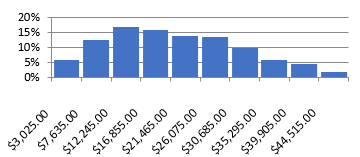
Figure 57 Probability Distribution Image 2
Each simulation generates 1,000 probabilities (individual values that are charted). The charts show how many of these probabilities fall into the range we declared when we entered the initial values. The simulation will never generate a probability outside the range we establish. In the left-side distribution, we see that a little more than 15% of the values are between 46 and 52, with more falling between 52 and 58. In the right-side diagram, only about 5% of the probabilities are between $3,025 and $7,635. These charts clearly show where the probabilities exist within the range we have established (or calculated).
Monte Carlo simulations use multiple probabilities to estimate potential outcomes.
These simulations are tools for estimating the probability of an outcome when the variables are random or unknown. These multiple probability simulations can be used to predict the probability of a vast array of outcomes, given the influence of randomized variables.
S. Ulam and Nicholas Metropolis first used the term Monte Carlo to describe the games of chance they saw in Monaco. Today, Monte Carlo simulations are used by stockbrokers, astronomers, meteorologists, navigators, and casinos, to understand probabilities under variable conditions.
Monte Carlo simulations produce probability distributions to display the range of probabilities. These statistical functions describe all possible variable values and likelihoods that a random value can take within a given range. These distributions evolved from observations in nature, giving some distributions preference in use in varying situations.
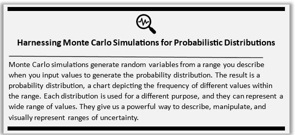
Figure 58 Harnessing Monte Carlo Simulation
Probability functions and distributions refer to the same thing but different parts. Probability functions are the mathematical formulas that drive the analysis. Probability distributions are the graphical representation of our executed probability function, often in charts or graphs. In this course, we use several common probability distributions, including:
-
- Triangular (3 values – minimum, most likely, maximum)
- Poisson (describes a large number of unlikely events that happen in a certain time interval)
- Pert (triangle weighted to the most likely)
- Bernoulli (estimates likelihood using hits and misses)
Triangular Distribution
The triangular probability distribution is a continuous probability distribution commonly used in statistics and probability theory. The distribution is defined by three parameters: a minimum value, a maximum value, and a mode. The mode is the value that occurs most frequently in the distribution. The distribution has a triangular shape, hence the name.
The triangular probability distribution was first introduced by R.A. Fisher, a British statistician, in his book “Statistical Methods for Research Workers” in 1925. Fisher used the distribution to model the uncertainty in estimating a population parameter based on a sample. The triangular distribution was used to estimate the range of possible values for the parameter based on the available data.
The triangular probability distribution is a useful tool for modeling situations where the data is limited, and the shape of the distribution is unknown. The distribution is particularly useful when the data is skewed, and the mean and standard deviation are insufficient to describe the distribution.
The distribution is defined by three parameters: a minimum value, a maximum value, and a mode. The mode is the most likely value of the distribution. The minimum and maximum values define the range of possible values for the distribution.
Pert
PERT (Program Evaluation and Review Technique) is a project management tool that helps to analyze and evaluate the tasks involved in a project. The PERT probability distribution is a statistical tool used in project management to estimate the probability of completing a project within a given time frame. The distribution is based on the PERT technique and is commonly used in project management.
The PERT probability distribution was introduced in the late 1950s by the United States Navy as a tool to manage the Polaris missile project. The distribution was developed to estimate the time required to complete a project based on each task’s expected time, optimistic time, and pessimistic time. The PERT probability distribution is used in various fields that require probability estimation, such as risk management, resource allocation, performance evaluation, and cost estimation.
In risk management, the PERT distribution estimates the probability of completing a task within a given time frame. The distribution is used to model the uncertainty associated with each task’s completion time and the project’s overall completion time.
The PERT distribution estimates the resources required to complete a particular task in resource allocation. The distribution is used to model the uncertainty associated with the completion time of each task.
The PERT distribution is used to evaluate a team’s performance in performance evaluation. The distribution compares the expected completion time of each task with the actual completion time.
In cost estimation, the PERT distribution estimates the cost of completing a task or project. The distribution is used to model the uncertainty associated with each task’s completion time and the project’s overall completion time.
Poisson
The Poisson probability distribution is a statistical tool used to model the probability of a certain number of events occurring within a specified time interval or space. The distribution is named after French mathematician Simeon Denis Poisson, who introduced it in the early 19th century.
Poisson developed the distribution to model the number of deaths by horse kicks among the Prussian army. He observed that the number of deaths followed a pattern of rare events occurring at random intervals. Poisson’s work on distribution laid the foundation for studying rare events in statistics.
The Poisson distribution is widely used in various fields, including finance, engineering, and physics, to model the occurrence of rare events. It is particularly useful when the number of occurrences is rare, but the probability of each occurrence is constant.
The Poisson probability distribution is a discrete probability distribution used to model the number of events occurring within a specified time interval or space. The distribution is defined by a single parameter, lambda (λ), representing the average number of events occurring within the specified interval.
The Poisson probability distribution requires one input parameter, lambda (λ), representing the average number of events occurring within the specified interval. This parameter can be estimated from historical data or expert opinion.
For example, in finance, the Poisson distribution can be used to model the number of credit defaults within a specified time interval. The parameter lambda can be estimated from historical data on credit defaults.
In engineering, the Poisson distribution can be used to model the number of failures in a system within a specified time interval. The parameter lambda can be estimated from historical data on system failures.
In physics, the Poisson distribution can be used to model the number of radioactive decay events within a specified time interval. The parameter lambda can be estimated from the decay constant of the radioactive substance.
Binomial Distribution
The binomial distribution is a probability distribution used to model the number of successes in a fixed number of independent trials, where each trial has only two possible outcomes: success or failure. It is a discrete probability distribution, meaning the possible outcomes are countable and can only take on certain values. Binomial distribution is widely used in statistics, especially finance, biology, and engineering.
The binomial distribution is defined by two parameters – the number of trials (#) and the probability of success in each trial (%).
The binomial distribution is like a game where you flip a coin a certain number of times and count how many times it comes up heads. Let’s say you flip a coin 10 times and want to know how many times it will come up heads. The binomial distribution can help you determine the chances of getting a certain number of heads.
For example, if you flip a fair coin (which means it has an equal chance of coming up heads or tails) 10 times, the chances of getting 5 heads are about 25%. The chances of getting 10 heads in a row are very low, about 0.1%.
The binomial distribution can help us determine the chances of getting a certain number of successes (like heads) in a certain number of trials (like coin flips). It helps us understand how likely something will happen and how much we can expect it to happen.
Generate Probability Distributions
In the tool kit, you get several triangular and pert distributions. These are provided so you can use them in analysis and for comparison. Entering the Min-ML-Max values for the designated data type will automatically generate (update) your probability distribution charts. (Fields in light yellow are data entry fields.). Notice that you can name these distributions to something meaningful for your analysis. Also, notice that each distribution is designated #, %, or $. This means that the distribution has been pre-formatted for this data type.
The tool generates 1,000 probabilities for each distribution. You can use the scroll bar to scroll through and see each of those 1,000 probabilities updated in the sparkline values.
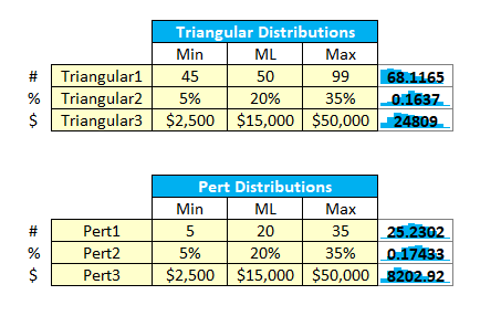
Figure 59 Triangular & Pert Distribution Input Screen
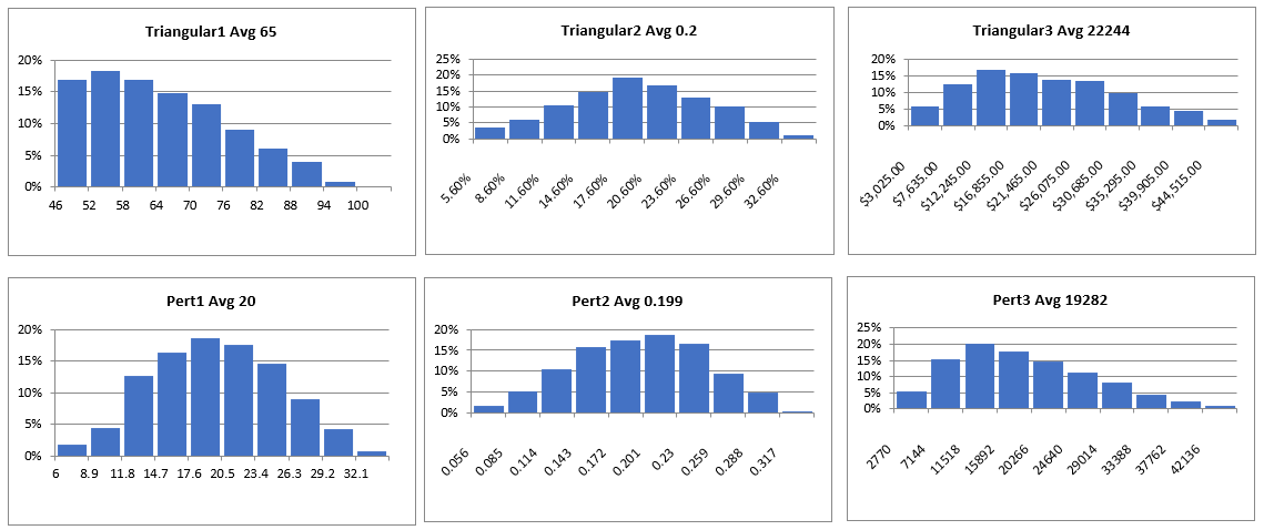
Figure 60 Triangular & Pert Distribution Charts
In addition, the tool allows you to multiply these probability distributions for use in your analysis. Note that we are multiplying full probability distributions, not multiplying the minimum values, most likely values, and maximum values. Multiplying probability distributions values will yield a similar, but slightly different results than if you multiply the individual values.
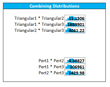
Figure 61 Combining Distributions
The results are also probability distributions with their own charts.
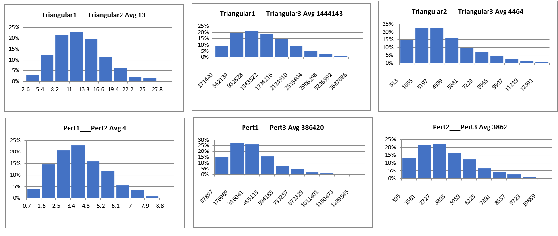
Figure 62 Combining Distribution Charts
The tool kit provides Poisson distributions to forecast several likely events.
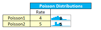
Figure 63 Poisson Distribution Interface
Your input is a rate value. This could be the average number of cyber-attacks observed over a period of several observed incidents. The meaning is specific to your analysis, as is the range of the time.
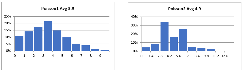
Figure 64 Poisson Distribution Charts
The Binomial distribution allows you to compare two items: perimeter strength and threat attacker strength. We have also given you a display of all the generated probability values for visual inspection. This way, you can gamify your analysis, pitting your security defense against an imaginary threat actor to simulate probable outcomes.
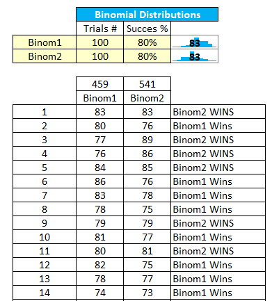
Figure 65 Binomial Distribution Input
The binomial distribution also generates probability distribution charts.
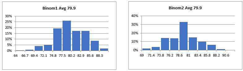
Figure 66 Binomial Distribution Charts
Using the Chart Area
After you have generated your probabilities, you will want to edit and customize the resulting charts. To do this, we recommend you COPY and PASTE the charts into the Charts tab leaving the original chart intact and in place for future updates.
FAIR Analysis Model
The FAIR™ (Factor Analysis of Information Risk) standard is a framework for quantifying and analyzing information risk consistently and repeatedly. The Open Group, a global consortium specializing in developing technology standards and certifications, developed the standard.
The FAIR™ standard provides a structured approach to information risk management that enables organizations to identify, analyze, and prioritize their information risks based on their potential impact on the organization’s objectives. The standard is based on the premise that information risk is a function of the likelihood of an event occurring and the magnitude of its impact.
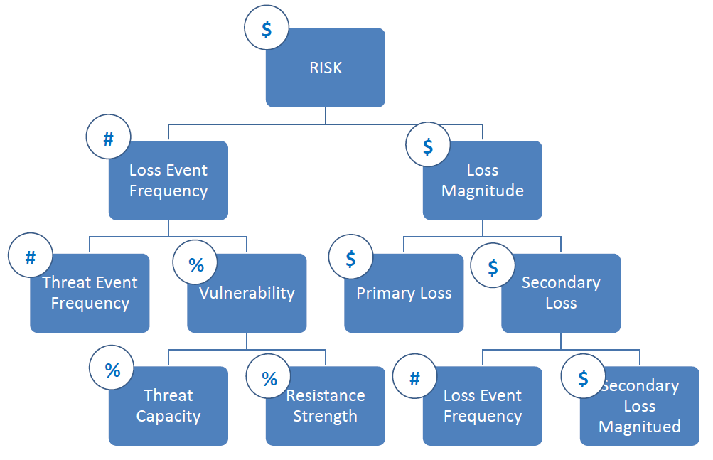
The Components of the FAIR™ Standard
The FAIR™ standard consists of six components that are used to quantify and analyze information risk:
Risk Scenarios: A risk scenario describes an event that could lead to a loss or impact on the organization’s objectives. Risk scenarios are used to identify the potential sources of risk and the potential consequences of those risks.
Threat Event Frequency: The threat event frequency is the estimated frequency with which a specific risk scenario could occur. This component is used to estimate the likelihood of a risk scenario occurring.
Threat Event Impact: The threat event impact is the estimated impact on the organization’s objectives if a specific risk scenario occurs. This component is used to estimate the magnitude of the impact of a risk scenario.
Vulnerability: A vulnerability is a weakness in a system or process that could be exploited by a threat actor to exploit a risk scenario. This component estimates the likelihood of a risk scenario being realized.
Control Strength: Control strength measures the effectiveness of the controls in place to mitigate a specific risk scenario. This component estimates the likelihood of a risk scenario being realized.
Risk Treatment: Risk treatment is selecting and implementing controls to reduce the likelihood or impact of a specific risk scenario. This component prioritizes the risks and determines the most effective way to manage them.
Figure 67 Expanding Risk Assessment: Beyond FAIR ™
While the FAIR™ standard provides many benefits to organizations that adopt it, some challenges are associated with its implementation. These challenges include:
Complexity: The FAIR™ standard can be complex and difficult to implement. Organizations may need to invest in training and expertise to implement the standard effectively.
Data Availability: The FAIR™ standard requires significant data to quantify and analyze information risk effectively. Organizations may need to invest in data collection and analysis tools to implement the standard effectively.
Organizational Buy-In: The FAIR™ standard requires organizational buy-in to implement effectively. Organizations may need to invest in change management and communication to implement the standard effectively.
The two main components of the FAIR™ Standard are FREE to download and available here:
- Risk Analysis (O-RA), an Open Group Standard (C13G), October 2013, published by The Open Group; refer to: www.opengroup.org/library/c13g
- Risk Taxonomy (O-RT), Version 2.0, an Open Group Standard (C13K), October 2013, published by The Open Group; refer to: www.opengroup.org/library/c13k
Download the FAIR ON A PAGE reference here: https://cdn2.hubspot.net/hubfs/1616664/The%20FAIR%20Model_FINAL_Web%20Only.pdf.
FAIR Analysis in Six Steps
The FAIR (Factor Analysis of Information Risk) standard is a quantitative framework for assessing and managing information risk. It provides a methodology for estimating the probability and impact of potential cyber-attacks, allowing organizations to make informed decisions about how to allocate resources and manage risk effectively.
The first step, scoping, involves defining the scope of the risk assessment, including the assets, threats, and scenarios that will be evaluated.
The second step, assessing the threat landscape, involves identifying the potential threats that could impact the organization, such as phishing attacks, malware infections, or denial of service attacks.
The third step, identifying risk scenarios, involves developing specific scenarios that describe how each threat could impact the organization. These scenarios should be realistic and based on historical data or industry trends.
The fourth step, estimating the frequency of loss events, involves assessing the likelihood that each risk scenario will occur. This involves examining the controls in place to prevent or mitigate the risk, as well as the external threat environment.
The fifth step, estimating the magnitude of loss events, involves assessing the potential impact of each risk scenario. This could include financial losses, reputational damage, or legal liability.
Finally, the sixth step, calculating the risk, involves combining the probability and impact estimates to arrive at a quantitative estimate of the risk. This can be expressed in financial terms, such as the expected loss over a given time period.
One of the key benefits of quantifying cyber risk in financial terms is that it allows organizations to prioritize their risk management efforts based on the potential impact of each risk scenario. By expressing the risk in financial terms, organizations can compare the potential impact of different risk scenarios and allocate resources accordingly.
Our Modified FAIR (tm)
The FAIR Standard includes two additional fields that we have removed from our model for simplicity. These fields are Contact Frequency and Probability of Action. These fields combined quantify the Threat Event Frequency. We removed these fields due to the complexity of estimating Contact Frequency. This allows us to more easily estimate Threat Event Frequency. Estimating Threat Event Frequency can be done by using the number of failed events. For example, the number of times a firewall blocked an attack, or the number of time end-point protection blocked malware. Given the FAIR definition of Vulnerability as the likelihood of a risk event being realized we maintain the joint probability between threat and likelihood.
Combining Probability Distributions
In our tools, probability distributions are stored as arrays, and as such, we can apply basic mathematical functions such as addition, subtraction, multiplication, and division.
The FAIR™ is a good example of how different values in probability distributions can be combined for analysis. For example, here are some ways FAIR combines distributions.
- A probability distribution of numerical data can be multiplied by a similar distribution of percentage values resulting in a numerical value distribution.
- Two probability distributions containing financial values can be multiplied or added.
- A probability distribution of numerical values can be multiplied by a distribution of financial values, resulting in a distribution of financial values.
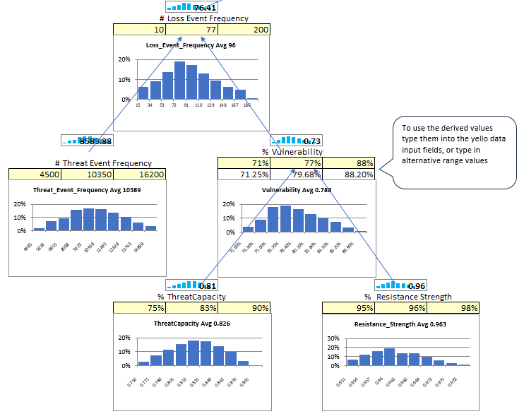
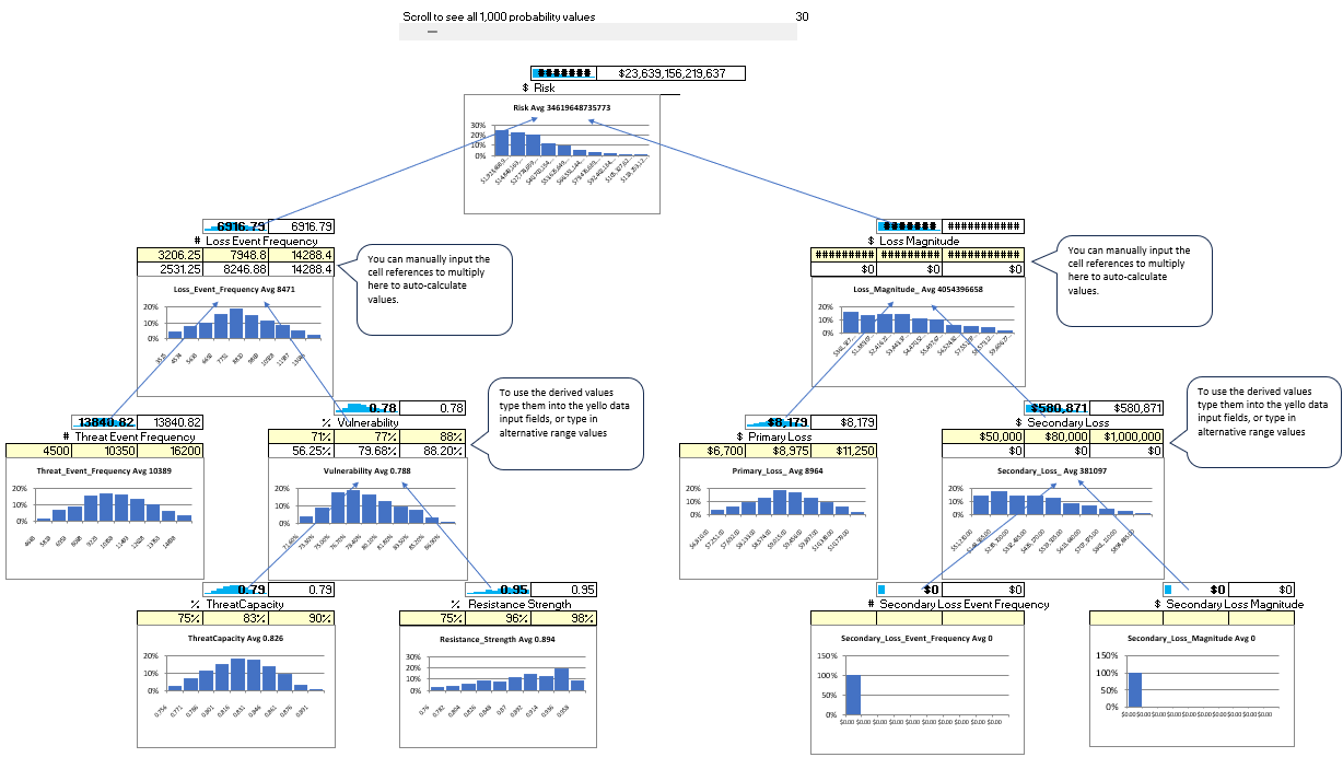
Within the tool, the FAIR™ model is presented on a single page. Here you can zoom into any component of the model and enter data or view the probability distribution chart.
Scrolling through, you can see the sparkline values rotate through all 1,000 probabilities for your model.
Within the tool, the FAIR™ model is presented on a single page. Here you can zoom into any component of the model and enter data or view the probability distribution chart.
Scrolling through, you can see the sparkline values rotate through all 1,000 probabilities for your model.
Derived Values vs. Direct Input
Some values in FAIR can be calculated directly (if you have data) or derived from data farther down in the model. Vulnerability is a value that can be entered directly or derived. Notice that the derived values are reflected, and you can use those values or overwrite and enter your own values. This is most helpful when there is insufficient data to derive a value. In such cases, enter the values at that level directly.